Why Meanline Scripting is Becoming Essential for Turbomachinery Design
Manual meanline design can sometimes feel less like design and more like managing a chain of tiny decisions.


Introduction:
With the advancements in computation power, optimization is not just limited to academics and research anymore. It can now be realistically used for industrial designs. There are several optimization software available in the market which utilize various powerful optimization techniques but not every software can be practical for industrial applications. This is especially true for the turbomachinery industry. Turbomachinery design is coupled with aero and mechanical optimization. The problems are highly constrained and usually involve non-linear functions. The optimization algorithm needs to be efficient to handle such problems.
Concepts NREC has partnered NUMECA International (now part of CADENCE Design Systems) to integrate their 3D Turbomachinery Design Software, AxCent™, with NUMECA’s optimization software, FINE™/Design3D to run CFD based optimization of turbomachines.
AxCent acts a parametric modeler in this environment and generates the necessary files needed for meshing. FINE/Design3D uses the optimization kernel, MINAMO, developed by CENERO based on the Design of Experiment (DoE) technique. MINAMO uses the advanced space-filling algorithm – Latinized Centroidal Voronoi Technique (LCVT) to generate the designs. The exploration of the design space is greatly sped up with a surrogate-based optimization technique. The surrogate model in combination with global optimization approaches (such as Evolutionary Algorithms) then uses an iterative process to find the global optimum.
Setup:
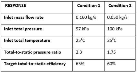
Engineers at Concepts NREC used AxCent and FINE/Design3D to perform a multi-point optimization of a radial compressor [1]. The base case was designed using a standard 1D manual design process based on the design requirements shown in Table 1.
As seen from Figure 1, the base case does not meet the design requirements at speeds 120,000 RPM and 170,000 RPM. Design points 1 and 2 are shown in blue and yellow dots, respectively.
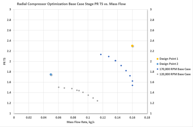
Figure 1. Base case design pressure ration vs. mass flow rate
An optimization study was set up using AxCent and FINE/Design3D running the FINE/Turbo CFD solver. The base case geometry is shown in Figure 2. The advantage of using AxCent as the parametric modeler is that it allows the use of ‘smart’ input variables as shown in Figure 2. When these smart input variables are varied by the optimizer, the neighboring hub and shroud contour points are also moved in a manner such the resulting geometry is free of any kinks and conserves the desired values of the additional input parameters Rex/R2, R3/R2, and PINCH. Additionally, the number of blades is also an input variable. An example of the application of these smart input variables and parameters is shown in Figure 3.
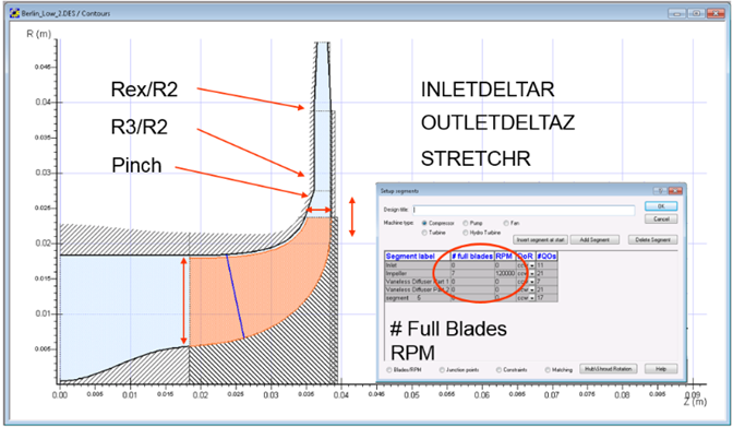 Figure 2. Contour and blade number inputs
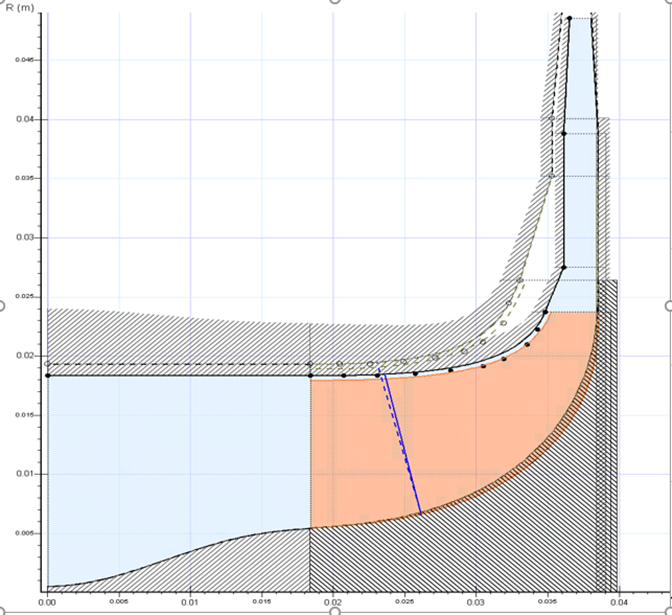 Figure 3. Solid lines/points = base case, dashed lines/hollow points = candidate design
FINE/Design3D also allows linking one input variable to another so that they vary relative to each other. This can be seen in Figure 4 which shows the blade angle distribution for the main blade. The independent variables are Beta1h, Beta1s, and Beta2s. The points circled in blue are dependent variables (linked to the independent variables through algebraic equations) and move relative to the independent variables to preserve the general curve shape.
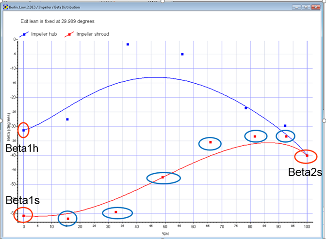 Figure 4. BETA blade angle inputs
After setting the upper and lower bounds for the input variables, a DoE of 51 designs including the base case was generated by running FINE/Turbo CFD solver to ensure there is an appropriate number of designs. The Latinized Centroidal Voronoi Technique (LCVT) was used as a space-filling algorithm to generate the designs.
The pressure ratio TS and Efficiency TS are the relevant responses from the DoE for both low and high flow rates. Figures 5 and 6 show the scatter plots for the same respectively.
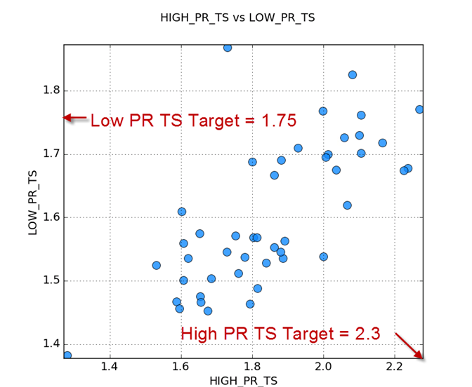 Figure 5. Scatter plot of PR TS from the DoE
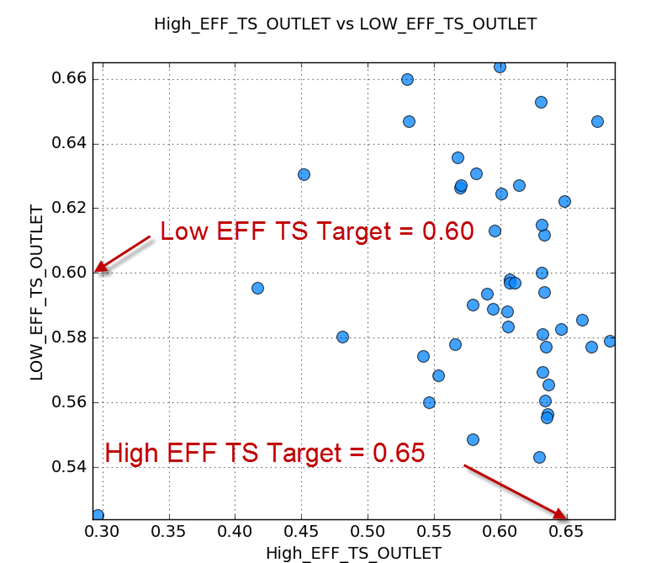 Figure 6. Scatter plot of Eff TS from the DoE
As can be seen from Figures 5 and 6, some designs meet the target for efficiency and low flow pressure ratio TS, but none meet the target for high flow pressure ratio TS. The goal of the optimization now becomes to mainly meet the target for high flow pressure ratio TS while still meeting the other design targets. Before moving on to the actual optimization using the surrogate model, MINAMO offers a slew of post-processing features that help understand the behavior of the input variables better.
Post-Processing the DoE Results:
One very useful post-processing feature offered by MINAMO is Leave-one-out (LOO) analysis. In this analysis, the surrogate model is formed but with one sample left out. This reduced surrogate model predicts the response for the left-out sample, and this is repeated for all samples and a correlation coefficient is formed. A correlation coefficient value greater than 0.5 is deemed sufficient to move forward with the optimization. Figure 7 shows the LOO analysis for high flow EFF TS and has a correlation coefficient of 0.639 > 0.5. The correlation coefficient for all other responses had a value greater than 0.5.
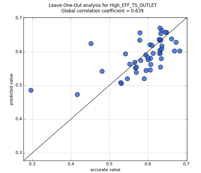 Figure 7. LOO Analysis for High Flow EFF TS
Another handy post-processing feature is Analysis of Variance (ANOVA) which uses the surrogate model to rank the percent impact of each input on a given response. The percentages are shown in a pie chart in which the size of the slice is based on the percent impact. Figure 8 shows the ANOVA analysis of PR TS at high flow. This shows that Impeller Exit Radius (R2), Backsweep angle (Beta2b), INLETDELTAR (R1t – R1H), and B2 have the highest impact on PR TS at high flow. ANOVA analysis for other responses is not shown here but the detailed analysis is given in [1].
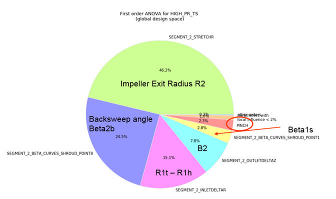 Figure 8. ANOVA analysis of PR TS at high flow
A trend of values for inputs and responses can be obtained using Self-Organizing Maps (SOM). These maps are contour plots of inputs and responses but have a unique feature – all the designs are displayed on the map (shown by small white dots) and always appear in the same position on every map. Figure 9 shows the SOM for PR TS at high flow and R2. The target value of PR TS at high flow is 2.3 and is shown in the lower-left corner of the map by a black circle. The corresponding map for R2 tells us that to achieve this target PR TS at high flow rate, the value of R2 should in range as shown by arrow on the map. SOM maps for all other responses and corresponding important input variables can be obtained similarly. These are not shown here but a detailed analysis is given in [1].
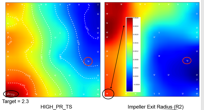
Figure 9. SOM for PR TS at high flow rate
After data mining the results from the DoE, it is clear that none of the designs meet the target value of PR TS at high flow. Several designs exceed the target value for PR TS at low flow and efficiency at both flow conditions. The optimization is formulated as follows:
Maximize PR TS at high flow rate with an upper bound of 2.3
Minimize PR TS at low flow rate with a target of 1.75
EFF TS (low flow) > 0.65
EFF TS (high flow) > 0.60
Global percent mass flow imbalance < 0.1 %
Percent CFD backflow at inlet or exit < 0.1 %
In addition to the constraints mentioned above, FINE/Design3D allows the user to write custom python scripts to add an additional check on the simulation results. In this project, a custom python script was written to monitor the RMS value of the global residual. Designs that fail to achieve a decrease of 3 levels of RMS residual error are marked as failed and removed from the database. The surrogate model is trained to steer away from zones of input variables that lead to simulation failure [2].
The scatter plots of PR TS and Eff TS at both flow conditions after the optimization search are shown in Figures 10 and 11 respectively. The base case is marked with a blue square, the optimal design is shown as the orange star. Designs generated by the DoE are shown in blue circles and designs generated by the search are shown in orange circles (large = feasible, small = unfeasible).
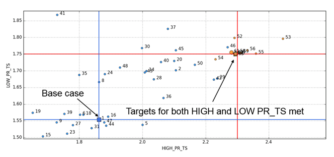 Figure 10. Scatter plot of PR TS search
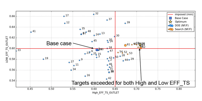 Figure 11. Scatter plot of EFF TS search
Magnifying either of the above plots shows that the optimal design is #57. This design meets PR TS targets (2.294 instead of 2.3 at high flow, 1.751 vs 1.75 at low flow) and exceeds both targets for EFF TS (0.708 vs 0.65 at high flow, 0.607 vs 0.6 at low flow). The optimization search obtained this result with just 6 additional runs past the DoE. This indicates the surrogate model is well trained.
Figure 12 shows a plot of accurate (CFD) value of PR TS at low flow vs that predicted by the surrogate model during the optimization search. It can be seen that from design 55 onwards the accurate and predicted values match closely. Other responses also show a similar behavior and are not shown here.
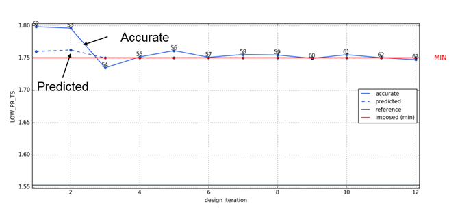 Figure 12. Accurate (CFD) vs. Predicted (Surrogate model) for PR TS at low flow
A meridional view of design #57 (dashed lines) overlaid with the base case design (solid lines) is shown in Figure 13. The input variables that have the most pronounced changes are R2, B2, and PINCH as anticipated from ANOVA. Figure 14 shows plot of beta distribution of hub and shroud for the optimal design (dashed lines) and base case design (solid lines). Compared to the base case values, BETA1s increased, BETA1H and BETA2B decreased. The main blade count for design #57 was 6 as compared to 7 for the base case.
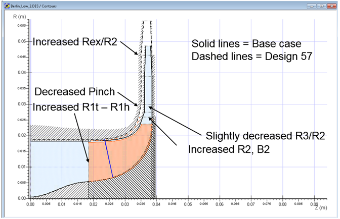 Figure 13. Overlay of contours of design #57 with the base case
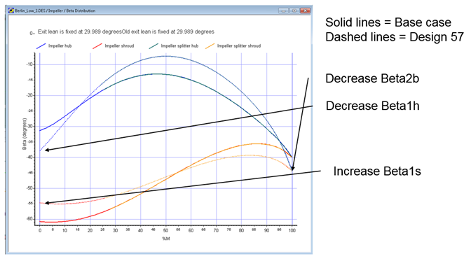 Figure 14. Overlay of BETA distribution for design #57 with the base case
A full performance map of design #57 and the base case is shown in Figure 15. There is plenty of margin on both stall and choke sides. In the realm of aerodynamic analysis, design #57 is hence acceptable.
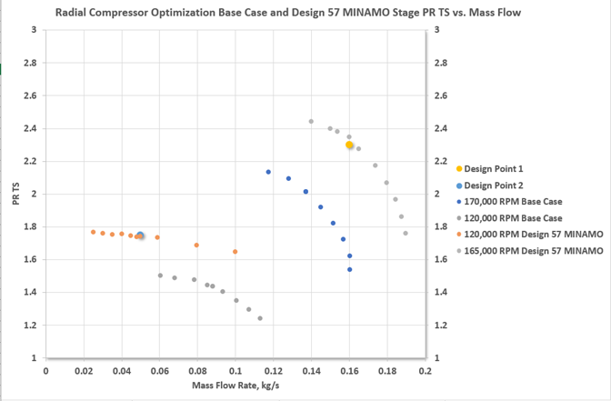 Figure 15. Full performance map for Design #57 and Base case – PR TS vs. Mass Flow
Conclusion:
This straightforward optimization (10 inputs, 1 objective aggregated from two PR TS targets, 8 constraints) was run on a modest single Windows workstation with 4 cores. The DoE was completed in about 48 hours and the optimization search in about 12 hours. Of the 51 DoE designs only 4 failed to converge, 1 failed to generate a valid mesh. Thus, the surrogate model was generated from 46 designs.
FINE™/Design3D coupled with AxCent™ is a robust optimization software bundle with several powerful post-processing features. The ability to run the search in parallel reduces the run time to weeks (in some cases even days) rather than months. FINE/Design3D also allows for customization of the project by allowing the designer to link custom python scripts. With AxCent as a dedicated turbomachinery modeler and AutoGrid as an automated meshing software for turbomachinery coupled with FINE/Design3D, this makes a fine choice for the turbomachinery design industry.
References:
[1] Edward P. Childs, Dimitri Deserranno, Akshay Bagi. “USING OPTIMIZATION IN INDUSTRIAL MULTI-POINT RADIAL COMPRESSOR DESIGN: MAP CORRECTION”, Proceedings of ASME Turbo Expo 2019: Turbomachinery Technical Conference and Exposition GT2019 June 17-21, 2019, Phoenix, Arizona, USA
[2] Baert L, Dumeunier C, Leborgne M, Sainvitu C, Lepot I. Agile SBO Framework Exploiting Multisimulation Data: Optimising Efficiency and Stall Margin of a Transonic Compressor. ASME. Turbo Expo: Power for Land, Sea, and Air, Volume 2D: Turbomachinery Paper GT2018-76639
[3] FINE/Turbo 13.1, NUMECA International
[4] FINE/Design3D 13.1, NUMECA International
[5] MINAMO, Cenaero
Do you have any questions, concerns or comments? Please let us know in comments section below or contact us at info@conceptsnrec.com
Tags: CAE Software, Optimization
Manual meanline design can sometimes feel less like design and more like managing a chain of tiny decisions.

For most turbomachinery engineers, optimization isn’t a new idea. It’s a critical part of their workflow that can’t be overlooked. But sometimes that crucial step isn’t easy to get to.
It’s no secret that turbomachinery design has been one of the most demanding CAE environments, thanks to tight tolerances, complex physics, and long design cycles. That hasn’t changed in 2026, but...