The Best CFD Averaging Methods for Distortion

Three-dimensional flow fields typically have some degree of distortion in the flow properties and flow profiles across a given cross section. These distortions can be quite significant in regions that include the exit plane of the impeller. Because most designers are interested in averaged values of performance, the question often arises as to what averaging technique is the best to use.

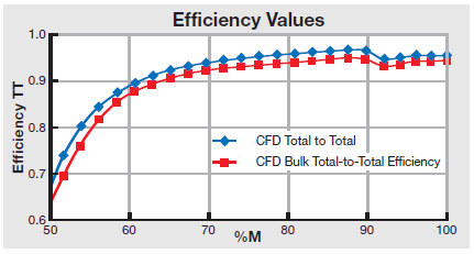
The plot above shows two methods of expressing efficiency in a typical radial compressor example.  In this case, the “Total-to-Total Efficiency” and “Bulk Total-to-Total Efficiency”.  The first represents the mass averaged efficiency of the various streamlines.  The second result is similar but efficiency is computed based on the separately mass averaged total pressure and temperature.  The results shown are not unusual. Typically, the difference between any two methods is at a maximum in the most distorted region, and they drift closer together as the flow fields mix out and flow unsteadiness, due to periodic rotating wakes, decays.

Although several averaging techniques are possible, there is no universally accepted or correct method of averaging. The three most common averaging methods are:  area, mass, and mixed out states.  Area averaging is probably the least often used method but is sometimes preferred for pressure since it conserves the net force on the surface.  Mass averaging is generally the most common method used and is more often than not the basis for quoted performance in testing and CFD results. The method for calculating a mass-averaged quantity is simple

where “i” is a cell face number on the cross-sectional area, and dm is the mass flux through the face.

The third option used for averaging is the mass-momentum-energy method (mixing to uniform flow state). Calculating this value is more complicated since an iterative method is needed in addition to some kind of equation of state for the fluid. Conceptually, during this type of averaging, non-union flow is converted to a uniform flow state across the averaging surface, while preserving the same mass flow, momentum flux in three directions, and energy flux as the distorted flow. There are actually two such flow states – one supersonic and one subsonic. The actual state reported is selected by calculating the averaged Mach number to determine which side of the sonic point is used. 

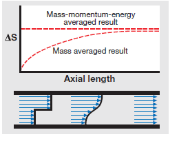
The mass-momentum-energy value is generally a more pessimistic number, but it is also a more conceptually representative number. Implicitly this number includes the effect of mixing loss that would be incurred when the non-uniform flow mixes out to a uniform state. The next figure shows a simple mixing problem in a frictionless duct. The flow, starting in the distorted state, mixes in the duct, and this irreversible process increases the entropy of the flow in the mass-averaged sense.  The mass-momentum-energy averaged  method incorporates the final potential  mixing loss implicitly. In essence, the  method mixes the flow and accounts  for this loss from the beginning, so no  change in entropy is seen.

So when comparing CFD results to test data, the “correct” averaging  method to use is the same method used for measuring and processing the test results. However, regardless of the test method used, it should be noted that in actual applications, the losses due to mixing of distorted flow are almost never avoided. While it is theoretically possible to recover the work from the various stream tubes without mixing them, this is almost never the case in practice. Inevitably, the stream tubes leaving the impeller will mix together and eventually impact performance. Using the mass momentum-energy averaging method effectively captures this effect.