Using Curvature Smoothing for Quality Reconstruction of Blade Sections Using Surface Data Tables

Frequently, there is a need to reconstruct 2D and 3D geometry from reported or measured surface data points. In most cases, the provided surface data include significant amounts of noise for various reasons, including quality of the scanned blade, deviations produced by the measurement system, curve digitization errors, data digital rounding and truncation, and errors in reporting the data.  This noise hampers quality surface reconstruction and masks the understanding of the design intent of the profiles.  It also affects the accurate representation of the geometry, manufacturing complexity, and aero performance which forms the basis on which a design engineer can execute any design improvements.

As an example, the plots in Figures 1-3 below show blade section contours, processed values of surface slopes, and curvatures for a nozzle section at the hub that was constructed using surface points reported in E3 HPT NASA CR-165608.

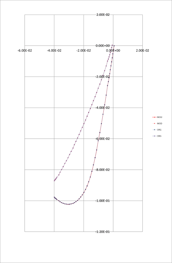
Figure 1. Blade Section Contours from Surface Data

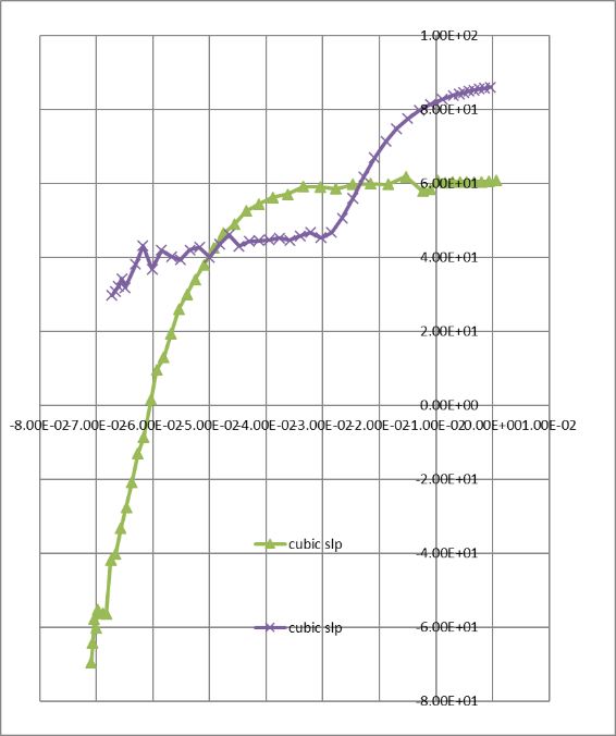
Figure 2. Surface Slopes

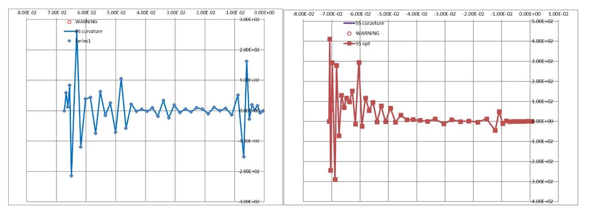
Figure 3. PS and SS Curvatures

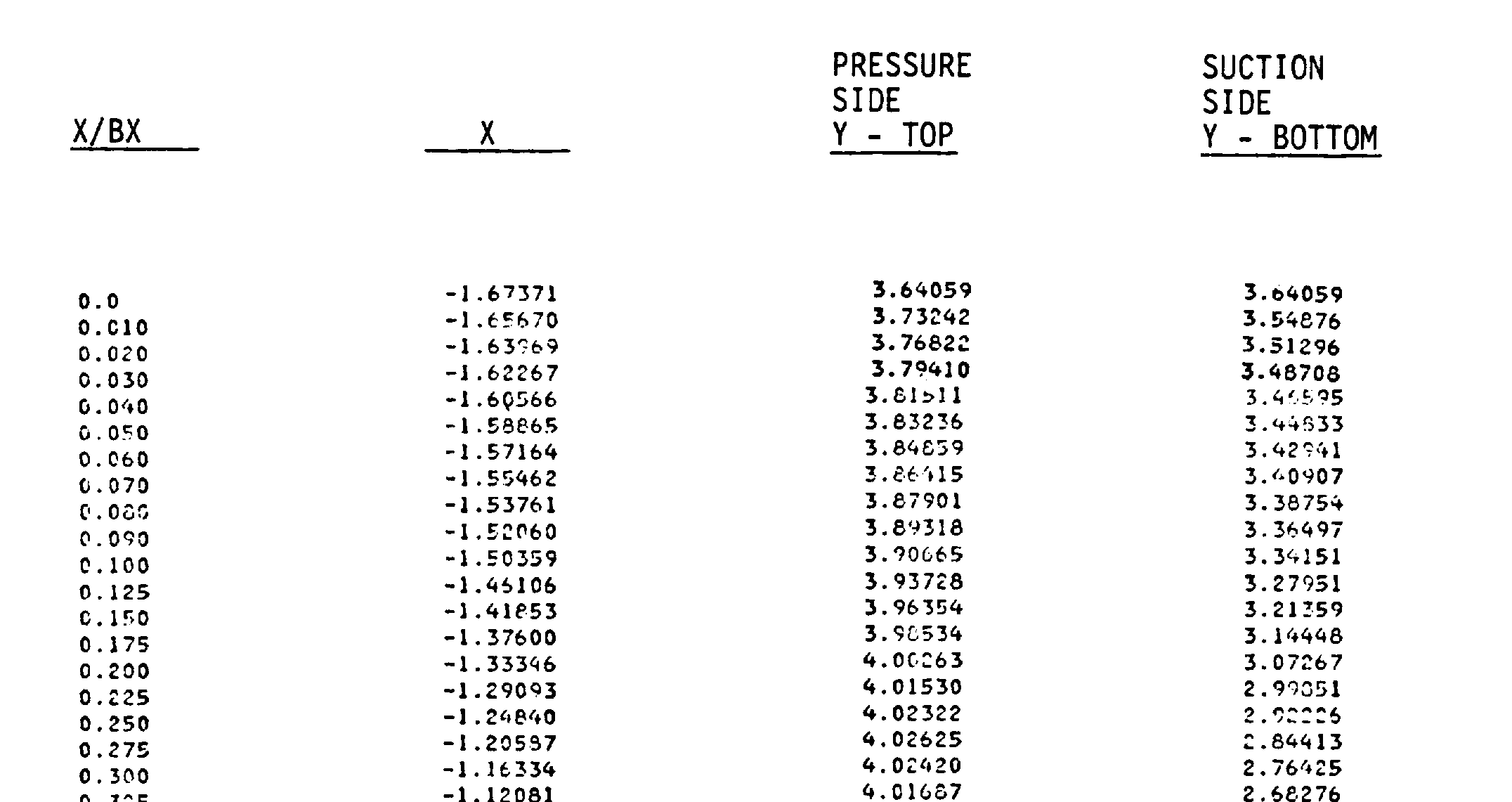
Though the blade section shape looks acceptable, the slopes and curvature plots show substantial geometry noise. In this example, the noise is due to errors in the surface data tables from OCR data processing of the NASA report, truncation, and rounding in the originally reported data. Here is a fragment of the data, for illustration:

As expected, the differentiation of the surface data in the slope and curvature calculations amplifies the noise. This makes de-noising the most noisy entity ( i.e., curvature distributions) the sensible primary target for surface data smoothing. Integration, reverse operation to differentiation, reduces noise levels in slopes and surface data, once curvatures are smoothed.

Simple polynomial smoothing to the curvature distributions could be applied in some situations, such as when the source data is for blades originally designed using polynomial/Bezier curves. However, polynomial fits may not work well if the blade curves are not of a single curve polynomial nature. In general, case blade surface curves can be spline curves of various types, including polynomials, trigonometric, lemniscates, circles, etc. Using Gaussian, running averages, or other filtering/smoothing methods can be used, but these usually require high density surface data to allow statistically robust averaging to work locally. This dense data may not always be available from the data sources.

Applying curvature smoothing, and integrating it to construct surface curves, may distort the blade section profile beyond the reasonable levels of the noise of the measured surface data.  In other words, removing noise in the curvatures does not guarantee the preservation of the profile shape in the local and global sense. To overcome this problem, it is necessary to restrict the local points to stay within allowable bounds, which are comparable with the magnitude of noise in the surface data and/or manufacturing tolerances, while performing smoothing operations. Some reference/critical points can be fixed in space to guarantee preservation of the blade shape.  In practical terms, this requires use of constrained optimization.

Constrained optimization requires a suitable smoothness criterion for the curvature distributions, which can work with arbitrary curves with either sparse or dense data tables.  A variety of optimization approaches were considered here at Concepts NREC, and tested on sets of practical profiles, including nozzle and rotor sections of gas and steam turbines with high-to-low reaction.

Staying with the example above, the following fits are reported using one of the non-polynomial smoothing approaches:

Figure 4. Smoothed Curvatures with Bounded Corrections in Surface Data (overlays vs. uncorrected curvatures)

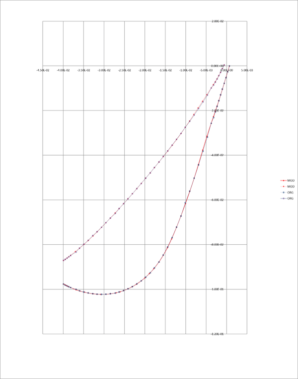
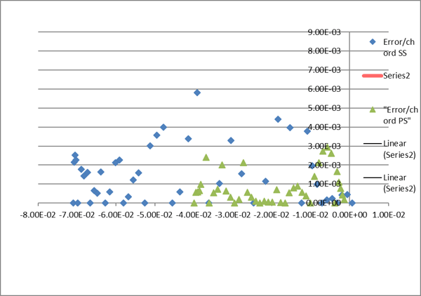
Figure 5. Overlay of the Smoothed Blade Section Shape over Original Data and Plot of the Applied Corrections to the Surface Data

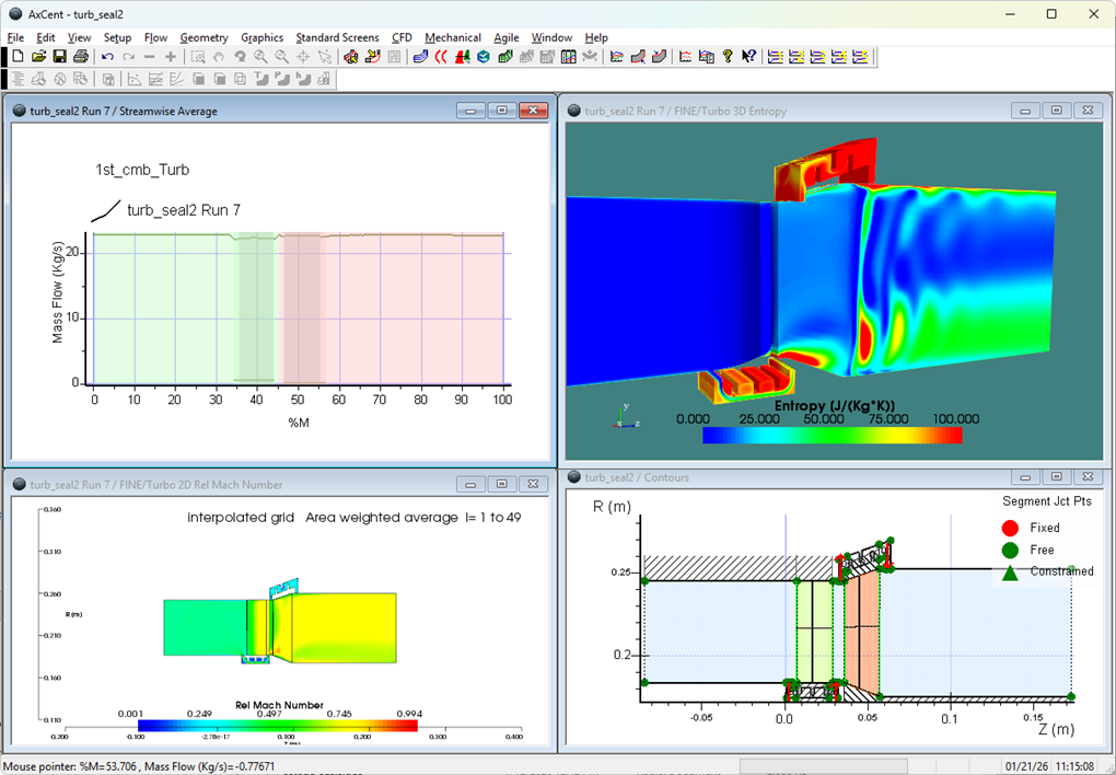
The geometrically smoothed geometry looks quite acceptable, with all adjustments staying within the allowed level of tolerance. To evaluate the benefits of the smoothed curvature reconstruction, original and smoothed blade sections were run in back-to-back (B2B) CFD using Axcent^®, Concepts NREC’s 3D geometry software:

Figure 6. B2B CFD Run for Original (top) and Smoothed (bottom) Profile

As expected, the B2B CFD showed cleaner loading distributions and lower loss by ~ 2.5%, for the smoothed profile vs. the original non-smoothed geometry.

To demonstrate the flexibility of this approach, the plots below show results of smoothing two Deytch turbine profiles, rotor and nozzle sections, reconstructed from sparse surface point data (<20 points per PS/SS curve).  These profiles are known to be constructed using patches of lemniscates, circles and straight lines, Therefore, there is no guarantee that polynomial fits are acceptable.

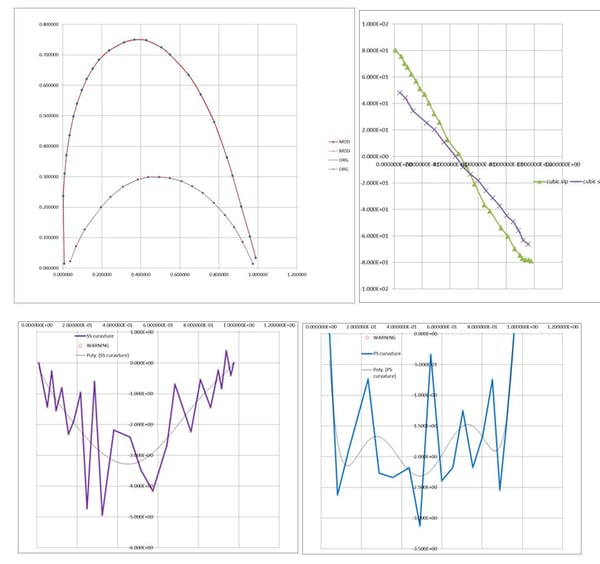
Figure 7. Original surface data, slopes and curvatures for rotor profile R2314 

 Figure 8. Constrained curvature smoothed profile (overlay), slopes and curvatures for rotor profile R2314A 

 Figure 9. Profile and curvatures for nozzle profile S9009A before (left) and after (right) constrained smoothing.

Note that, in this example, the polynomial curvature fit over the original data on the suction side; the black trend line, in the top-left plot, fails to catch the expected about-constant curvature domain at the exit of the suction side curve (top-right plot).  Conversely, the smoothing using constrained optimization captures that behavior very well.

It is worth mentioning that the use of blade section smoothing can help reverse engineer historical and measured data to construct curvature-defined profiles, which can be stored in a library of profiles. These stored profiles can be reused directly or indirectly (as sources of rules) in any new design projects. This feature, called Profile Repository, can be found in both AXIAL™ and AxCent software modules in the Agile Engineering Design System®, from Concepts NREC.